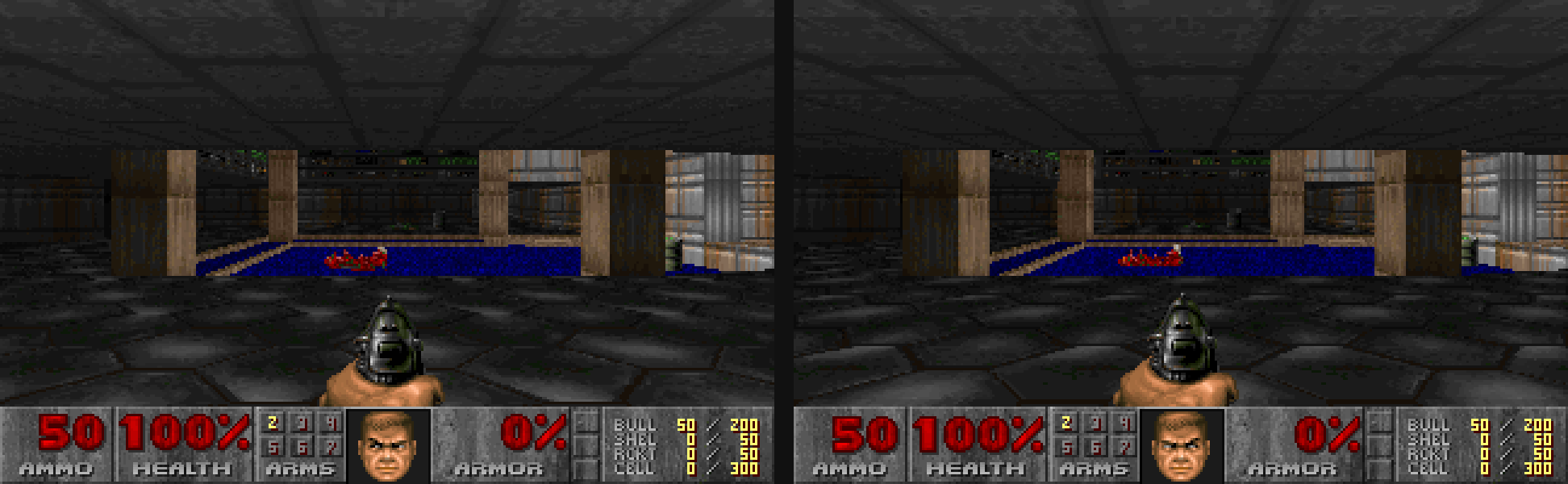
TL;DR: We ported the original 1993 Doom’s game logic and renderer to SQL and ran it inside a database. The game loop runs at the original 35 FPS, while the renderer produces the complete 320x200 frame buffer at up to 60 Hz on my Laptop. Python only handles timing, reads the keyboard, and displays the bitmap it gets back. Multiplayer also works.

You can play it right now Deathmatch, four slots, first come first served.

SQLDoom on 🇪🇺 EU Servers

SQLDoom on 🇺🇸 US Servers

It’s the shareware version of the first episode. If all seats are taken, you land in the queue. If the queue is full, you can still poke around and query live game state via SQL while you wait.

SQLDoom

Last year, I published DOOMQL [Github]. It rendered some ASCII-art roughly resembling Doom at 30 FPS and people liked it a lot. But some people correctly pointed out that it is a lot closer to Wolfenstein 3D than Doom, since it uses a raycasting approach. Doom, on the other hand, uses BSP trees, which make correct depth ordering cheap enough to afford textures, arbitrary wall angles, and varying floor heights.

Well I couldn’t let this rest and after some tinkering (you guessed it, parental leave again), I can finally present the real Doom running entirely in SQL.

The rules

Let’s first establish a few baseline rules about what we want to achieve:

1. It should look like the real Doom. DOOMQL’s visual fidelity is pretty embarrassing in hindsight.
2. But more importantly, it also should feel like the real Doom. The original game is just raw fun.
3. The rendering must be purely SQL-based. The only acceptable SQL output is a table or a bitmap encoding exact RGB values for every pixel.
4. The game loop must also be purely SQL-based. It’s okay to use user-defined-functions inside the DB, though.
5. I’m allowed to write a client in another programming language, as long as it only takes care of parsing the input, driving the game tics, and rendering the output bitmap.

Architecture

Python is delibarately boring (Rule 5). A single script uses pygame to drive input, draw the output bitmap and trigger a game tic 35 times a second. Game logic, game state, and renderer live inside the database.

                         Python
                 input / timing / display
                    |              ^
                    |              |
          run game tic        request frame
                    |              |
                    v              |
          +----------------+  +----------------+
          |                |  |                |
          | SQL game logic |  |  SQL renderer  |
          |                |  |                |
          +-------+--------+  +--------+-------+
                  |                    ^
                  |                    |
                  v                    |
             +-----------------------------+
             |                             |
             |       game state tables     |
             |                             |
             +-----------------------------+

The two paths are intentionally separate: The game logic runs on a fixed 35 Hz loop, while the renderer is a pure function of the game state tables and the client can ask for a new frame whenever it wants (i.e., as fast and often as possible).

Loading the Game Data

Conveniently, Doom’s .wad file format is actually is highly relational already.

Two VERTEXES are connected by a LINEDEF, which has two SIDEDEFs. SIDEDEF bound a SECTOR which can have THINGS in them, you get the idea. Translating the whole WAD into a database was surprsingly straightforward and took about 1000 lines of Python. Importing all of Doom 1 takes about 18 seconds on my laptop.

For example, here’s a query rendering E1M1 from a bird’s eye view:

WITH wall AS (
  SELECT round((v1.x + (v2.x - v1.x) * t / 32.0) / 48) AS col, -- 48 units per column
         round((v1.y + (v2.y - v1.y) * t / 32.0) / 96) AS row, -- chars are 2:1
         l.left_sd_id < 0 AS solid -- one-sided lines are pass-through
  FROM linedefs l, generate_series(0, 32) AS t        -- walk each line in 32 steps
  JOIN vertexes v1 ON (v1.map_id, v1.id) = (l.map_id, l.v1_id)
  JOIN vertexes v2 ON (v2.map_id, v2.id) = (l.map_id, l.v2_id)
  WHERE l.map_id = 1
)
SELECT string_agg(CASE WHEN (col, row) IN (SELECT col, row FROM wall WHERE solid) THEN '#'
                       WHEN (col, row) IN (SELECT col, row FROM wall)             THEN '.'
                       ELSE ' ' END, '' ORDER BY col)
FROM generate_series(-16, 79) AS col, generate_series(-51, -21) AS row
GROUP BY row ORDER BY row DESC;

Output:

                                                 #####################
                                                 # ..................#
                                                 # . ......         .#
                                                 # . ...... ######  .#
                                              ######         .. ##  .#
                                          #####..  .         .. ##  ##
                                          #  ####### ...... ######  ##########
                                          # ##   # .                ###..  ..##
  ################                       ## #    ###.........######## #####.  ##
###  ........... #                ########..########.........###         #### .##     ######
#  ..           ##########     ####         ##                 ##        #..... #######    ##
#  .          #####  ... ##  ###   #.....#..##    ........      ##########..... ....##.#### ##
#  .     ###.###  ......  ###  .   .        ##  ...      ...             . ......     .#  ##  ##
#  .     ##..  .  ......  ##   .   .        ##  .           .            . ..........  ##  ## ##
#  .     ###.######  ...  ######   #.....#..##  ...        ..            #.    ... ..   # ## ##
#  .           ############    #            ..    ..........             #.......... ...# #  #
###.........     #             #####     #####                           ##..... ... ##.###  #
  ################                 #######   ####.........##.##........####### .#######  ### #
                                                 ###########.#################  #  ####  # # ##
                                                           #.#      ####......  #  # .   ### ##
                                                           #.#################  #  ###########
                                                           ####. .####       #..#
                                                              #####     ######..######
                                                                        #   .    ..  #
                                                                        #   ##...##  #
                                                                        #   ##   ##  #
                                                                        ######..######
                                                                             ####
                                                                             #####
                                                                             #.. #
                                                                             #####

The Game Loop

It was important to me to actually port Doom, not only render frames that vaguely look like it. Of course, the visuals play a big part in that, but Doom also just feels awesome to play. Take a look at the following scene which is rule 2 in action (me having fun):

As you can see, there is a lot going on. Just in this short clip we see:

• Player input has to be polled and processed (walking, turning, shooting),
• enemies walk and attack,
• items are picked up,
• the rocket launcher fires projectiles that move,
• rocket explosions have a blast radius,
• enemy sprites have to be rendered,
• animations, view bobbing, and the HUD

And we don’t have a lot of time to process all of it: The original Doom ran on a fixed 35 Hz clock, so a tic has a budget of 1000 ms × 35 Hz = 28.6 ms. It also drew exactly one frame per tic, so it was capped at 35 FPS as well.

SQLDoom keeps the game logic at 35 Hz (so all the original constants still work), but decouples the drawing. The client can query (get it?) for a frame whenever it likes and we interpolate the camera position between tics. So there are two budgets we have to take care of:

• Running a tic every 28.6 ms (or it will feel just completely wrong)
• Rendering at least 35 frames a second (less is kind of okay, but won’t feel smooth)

The tic sequence

Game tics are inherently procedural. We have a sequence of things we have to do each time we run the tic. CedarDB has a scripting language called cedarscript, it closely resembles PL/pgSQL and allows us to plan beforehand what to do each tic.

Here is a small section of the tic function:

doom_cs_clock(map, p);
let mut plan = doom_cs_plan(map, p);    -- returns a bitmask of functions to trigger

let use_queued = doom_tic_use(map, p, plan);
if (plan & 2) <> 0 OR use_queued { active = doom_cs_activate_specials(map); }
if (plan & 4) <> 0 OR active <> 0 { doom_cs_doors(map, p); }

doom_tic_move(map, p);                  -- full movement, or just turning
doom_cs_death(map, p);                  -- process deaths

plan = doom_cs_plan(map, p);            -- the world moved; re-plan
plan = doom_tic_secrets(map, p, plan);  -- secrets, walkover lines, pickups
plan = doom_tic_weapon(map, p, plan);   -- weapon state, hitscan, damage
...
if sound_due { doom_cs_sound(map, p); } -- yes, we also play sounds
doom_cs_monsters(map, p);               -- always
doom_cs_sector_fx(map, p);              -- always
doom_cs_thing_physics(map);             -- always

The python driver from above calls SELECT doom_run_game_tic(...) every 1/35 second.

Each of those called functions then execute a batch of SQL statements. Below is a part of the state machine of the monster AI.

-- Abridged from sql/runtime/functions/26_cs_monsters.sql.
WITH RECURSIVE
  monsters AS ( [...] ),   -- who is alive, what kind, where
  los      AS ( [...] ),   -- visible, in_view_cone, dist: recursive, walks walls
  decision AS ( [...] ),   -- one row per actor: its state and what it can see
  transitions AS (
    SELECT d.*,
      CASE
        WHEN NOT d.alive AND d.state NOT IN ('die', 'dead', 'xdeath') THEN
          CASE WHEN d.health < -d.max_health AND d.xdeath_frame IS NOT NULL
               THEN 'xdeath'::actor_state ELSE 'die'::actor_state END -- GORY EXPLOSION!
        WHEN d.state = 'stand' THEN
          CASE WHEN d.visible AND d.in_view_cone AND d.dist <= sight_range
               THEN 'see'::actor_state ELSE 'stand'::actor_state END
        WHEN d.state_tics > 1 THEN d.state          -- animation still running
        WHEN d.state = 'see' THEN
          CASE WHEN d.visible AND d.dist <= d.attack_range
                    AND d.attack_cooldown <= 0
               THEN 'missile'::actor_state ELSE 'see'::actor_state END
        [...]                -- die, xdeath, missile, pain, barrel: 5 more
        ELSE d.state
      END AS next_state
    FROM decision d
  )
UPDATE monster_ai ai
SET state = n.next_state, state_tics = n.next_tics, seq_index = n.next_seq,
    fired_this_tick = n.advances AND n.lands_on_attack_frame
FROM next_values n
WHERE ai.map_id = n.map_id AND ai.thing_id = n.thing_id;

As you can see it encodes the behavior of the clip above: If an enemy takes extreme amounts of damage (CASE WHEN d.health < -d.max_health AND d.xdeath_frame IS NOT NULL) it violently explodes! (THEN 'xdeath'::actor_state).

Tic driver performance

Here’s a waterfall rendering of a game tic:

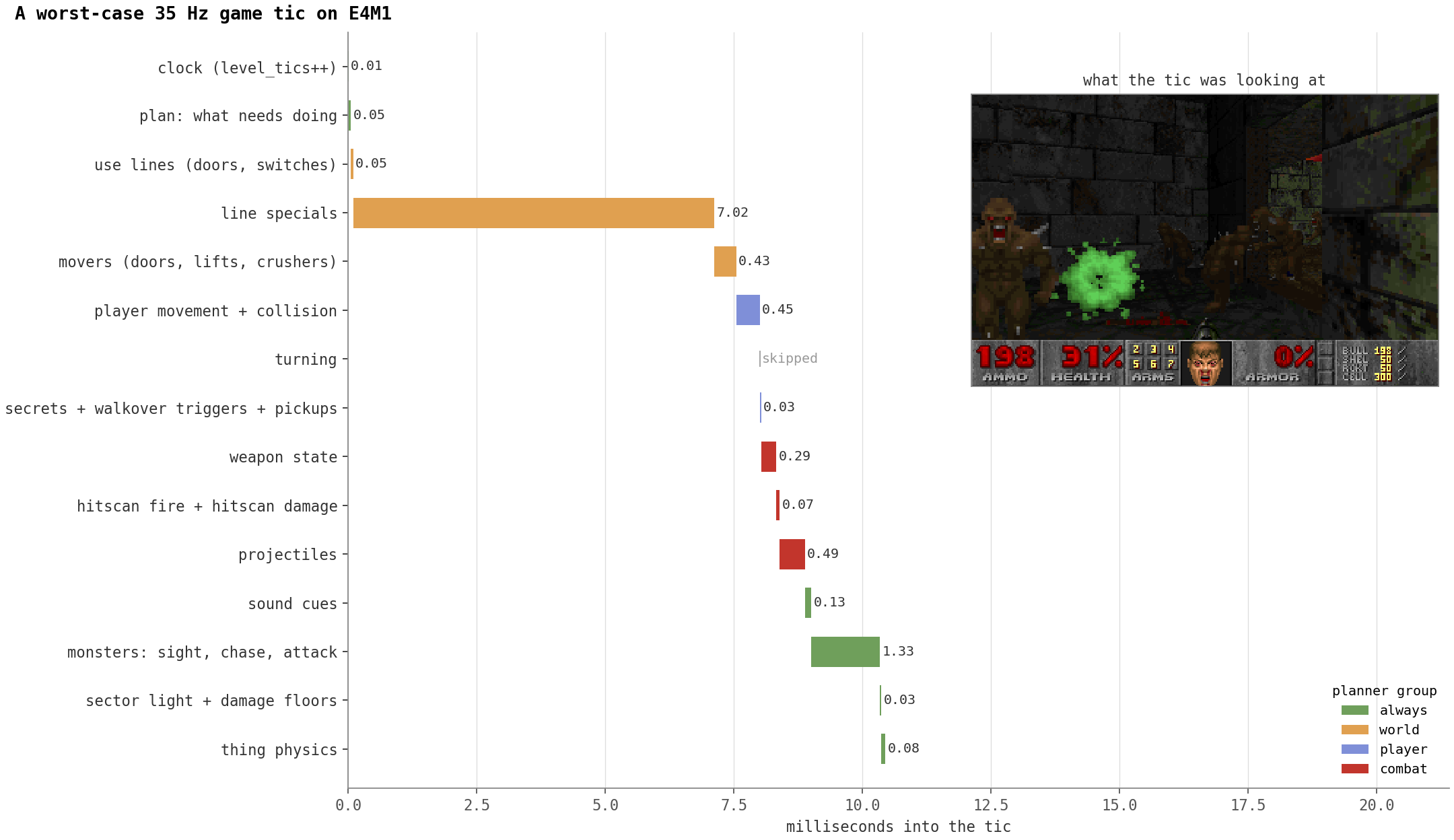
It’s actually the slowest game tic I was able to find. It’s in level E4M1 with 46 awake monsters all trying to rush at me through a currently opening door. It takes 10.45 milliseconds, so ~37% of the available tick budget.

A more typical tic with 6 monsters awake takes 2.15 milliseconds on average, or about 8% of the budget. Lots of headroom to spare!

To be honest, I was surprised how easy it is to express pretty complicated game logic in SQL. The game logic is just ~5900 lines of SQL. While this sounds a lot, it’s definitely less than the original C source code which does the same in about 9000 lines!

Also, it forces you to think differently. Instead of iterating over, e.g., enemies one-by-one you just write a simple UPDATE ... WHERE condition and let the database figure out how to best apply that - in parallel, automatically!

That also finally made the Entity Component System (ECS) pattern click for me. Here, each entity (player, monster, thing, …) has multiple components (position, sprite, stats, …) and a system (monster ai, move player, damage calculation) decides on how entities with a given set of properties interact with each other. ECS is a lot about data locality and how to iterate over entities that have a given set of components. Well, in SQL we are very used to data intensive processing! Every component becomes a table, and every system becomes an update or insert that just joins the tables it’s interested in with the entity as join key!

Rendering

Every frame is just a giant view that reads the level geometry and game state plus the player position as input and returns a complete framebuffer. Here’s a sketch of the whole rendering pipeline:

WITH RECURSIVE
  render_context AS (SELECT $1 AS map_id, $2 AS player_thing_id, $3 AS difficulty),
  pos            AS (SELECT $4 AS x, $5 AS y, $6 AS z, $7 AS angle),
  visible_children AS ( ... ),    -- walk the BSP, culling invisible segments
  clipped, projected, on_screen,  -- project segments to screen space
  wall_parts, columns, fragments, -- one row per wall pixel
  panel_clips, plane_spans, ...,  -- ceiling/floorclip as window functions, visplanes
  thing_pixels, sprite_fragments, -- sprites
  fragment_union, resolved,       -- every candidate pixel, resolve for the nearest
  view_colored, ui_colored,       -- COLORMAP, status bar
  framebuffer AS ( ... )          -- 64,000 rows of (x, y, rgb)
SELECT string_agg(rgb, ''::bytea ORDER BY y, x) AS frame_rgb
FROM framebuffer;                  -- 192,000 bytes, one row

The implementation is ~1300 lines of SQL (excluding comments) spread across 89 CTEs, so pretty complicated for a SQL query!

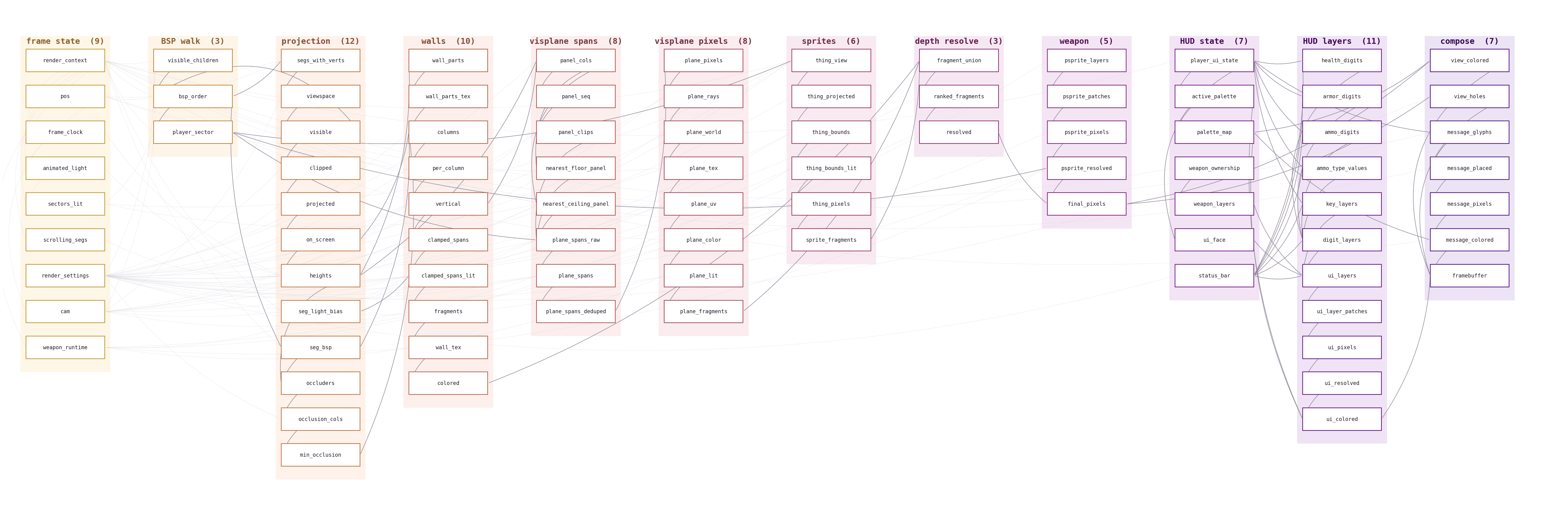
But despite looking like complete insanity, this pipeline is actually pretty close to what Doom does. SQL even has one advantage: The linux_doom source uses about 3300 lines (excluding comments) for its rendering engine. About 2.5x more lines than SQLDoom. Whether it was a good idea in the first place is a different question, and we’ll talk about that later.

Let’s first look at the most interesting parts of the rendering pipeline:

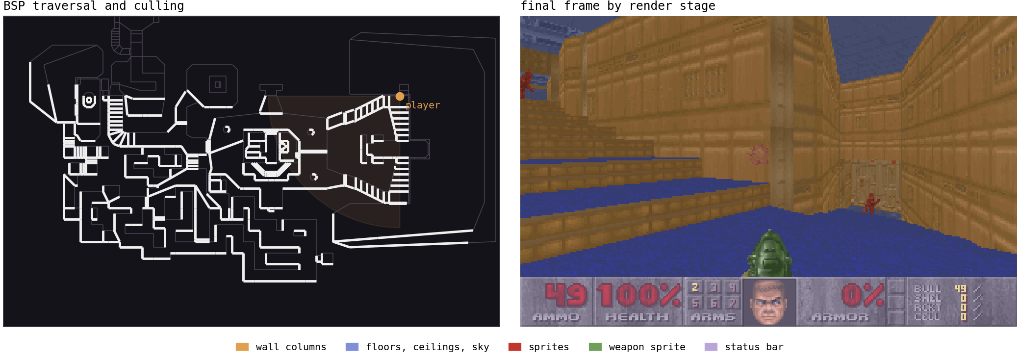
The left half shows bsp-based culling, the right half visualizes wall rendering and visplanes.

BSP traversal

Since nobody in 1993 had GPUs with hardware-accelerated Z-buffering, Doom had to get occlusion right by drawing in the correct order. The way Doom does it is pretty ingenious: It paints front to back and keeps track of which pixels it already painted (i.e., if I have already drawn a wall pixel, I don’t have to draw the monster behind it). But that’s easier said than done: We need an efficient way to order everything in the level by depth.

Doom gets this ordering by using precomputed BSP Trees baked into the doom.wad file. Every node of the tree is a line splitting the map in two. The map’s sectors thus get chopped up into a lot of subsectors which are on either side of those lines, and are then inserted into the tree so that we get the following properties:

1. each subsector is a leaf and
2. each subsector is convex (i.e., you can see any wall from anywhere inside it)
3. at every tree node, the entire subtree that is on the camera’s side is guaranteed to be in front of the subtree on the other side.

By recursively traversing the BSP tree, we thus get a front-to-back order of all subsectors. This gives us the rendering order directly: Once a screen region has been covered by something nearer, objects behind it can be skipped.

Here’s how this looks like in motion (you might have to view it in full screen):

On the left, subsectors are ordered front to back, while BSP branches out of view are eagerly culled. In the middle you can see the order that SQLDoom assigns each region. On the right, you see the resulting frame with walls colored according to the subsector they’re in.

The middle panel shows an optimization SQLDoom makes: For better performance we pre-compute all paths in the BSP tree once at load time. For a given position, every step along such a path is either taking the front (encoded as 0), or the back (encoded as 1). If we pack these decision into a bigint, and sort that lexicographically (order by), we get the right front to back ordering.

SELECT ssector_id, ROW_NUMBER() OVER (ORDER BY sort_key) AS bsp_seq
FROM (
  SELECT st.ssector_id,
         -- back = 1 at bit (40 - depth), front = 0.
         SUM(CASE WHEN st.side = fs.front_side THEN 0::bigint
                  ELSE (1::bigint << (40 - st.depth)) END) AS sort_key,
         BOOL_AND(vc.keep) AS visible   -- was any parent bbox culled?
  FROM node_path_steps st -- materialized view, every root-to-ssector path
  JOIN nodes n ON ...
  CROSS JOIN LATERAL (SELECT ... AS front_side) fs -- on which side are we?
  JOIN visible_children vc ON ...
  GROUP BY st.ssector_id
) s WHERE s.visible;

One sum() ... order by replaces the whole recursive descent! 40 bits should also be able to handle any map we throw at it: The deepest BSP-Tree is that of E4M8 and has just 32 levels. As long as your maps aren’t larger than 256 times the biggest vanilla map, you’re all sorted!

If you look carefully, you can see that our bsp traversal also handles culling: Conveniently, every node in the .wad also defines a bounding box of all of its children. If we can prove that our view frustum is entirely outside of that bounding box, we don’t have to consider that subtree for rendering - that is what visible_children.keep signifies. bool_and(vc.keep) thus drops all subsector where any ancestor doesn’t qualify.

Everything afterwards in the pipeline is just joined against bsp_seq so only visible subsectors are considered and in the right order.

Walls and Visplanes

Doom is kind of cheating, it looks 3D, but in reality it’s a 2.5D game. It’s essentially just a flat surface with perfectly vertical walls and ceilings always being parallel to the ground. This makes rendering far easier than in a real 3D engine:

1. Paint all walls (front to back, as discussed)
2. Everything that isn’t painted yet, is either a floor or a ceiling. Paint that.
3. Sprites (monsters, barrels, pickups) are flat images that always face you (think cardboard cutouts), so no complicated transformations here (except for when they overlap a wall, but we’ll get to that).

Walls

A wall occupies a set of contiguous screen columns, and within each column it is a contiguous span of pixels. So we can just paint walls one-by-one, front-to-back by expanding rows and columns via generate_series():

columns AS ( -- emit a row per screen column the wall w covers
  SELECT w.*, x AS col_x, ...
  FROM wall_parts_tex w
  CROSS JOIN LATERAL generate_series(
    GREATEST(0, FLOOR(w.screen_x1)::int),
    LEAST(screen_w - 1, CEIL(w.screen_x2)::int)) AS x
),
fragments AS ( -- one row per pixel the wall covers in this column
  SELECT c.col_x AS x, y, c.depth_x AS depth, c.u_i, c.v_i
  FROM clamped_spans c
  CROSS JOIN LATERAL generate_series(c.y_start, c.y_end) AS y
)

Doom uses two loops instead: R_RenderSegLoop to get the screen columns and R_DrawColumn to draw the pixels.

Rendering the walls cost us on average 1.7 ms.

Visplanes

Now that we have the walls out of the way, let’s talk about the fun part: The floors and ceilings, what Doom calls visplanes.

Unfortunately, Doom’s rendering algorithm doesn’t translate to SQL nearly as well since it’s highly imperative: Doom keeps two arrays, ceilingclip and floorclip which have one entry per screen column. They mark the band in each column that is still open (i.e., has to become floor or ceiling and hasn’t been painted yet) Whenever a new wall is painted, they are mutated until every pixel is filled. Not only does Doom mutate them, but it’s also very important to mutate them in the right order. It’s ingenious! In the end it’s just a flood fill algorithm, but everything looks 3D basically for free (in C, that is).

SQLDoom has to approach this problem differently, as we don’t have the concepts of loops or mutable state in SQL. So instead of looping, we turn to sorting and aggregating over those sorted runs - a poor man’s loop!

The things we iterate over here are called panels: One part of a wall appearing in one column of the screen. Some panels draw something: a solid wall (solid), the wall above a door (upper), or the wall part below a window or a parapet (lower), some panels are just there to influence how other panels are rendered: If you step out of a door below a balcony, there’s something above you and that has to end somewhere.

So for each screen column (col_x) we have an ordered list of panels from near to far. The clip state before a panel is thus defined entirely by the row preceding it. Do I smell window functions?

Since this is pretty hard to explain in text, let’s watch a video instead!

Here’s the (abbreviated) SQL query:

panel_clips AS (
  -- 1. the band as the NEARER panels left it
  SELECT p.*,
    COALESCE(MAX(CASE WHEN part IN ('solid','upper','upper_flush')
                      THEN y_bot::int + 1 END) OVER w, 0)            AS cc_before,
    COALESCE(MIN(CASE WHEN part IN ('solid','lower','lower_down')
                      THEN y_top::int - 1 END) OVER w, screen_h - 1) AS fc_before
  FROM panel_seq p
  WINDOW w AS (PARTITION BY col_x ORDER BY depth_x, bsp_seq, part, seg_id
               ROWS BETWEEN UNBOUNDED PRECEDING AND 1 PRECEDING)
),
plane_spans_raw AS (
  -- 2. whatever the band leaves uncovered is a ceiling above the wall...
  SELECT col_x, fsec AS sector_id, f_ceil AS plane_z, 'ceil' AS plane,
         cc_before         AS y0,   -- from where nearer walls stopped
         f_ceil_y::int - 1 AS y1    -- down to this panel's own ceiling
  FROM panel_clips
  WHERE part IN ('solid','upper','upper_open','upper_flush')
    AND f_ceil_y::int - 1 >= cc_before          -- nothing left open: skip
  UNION ALL
  -- ...and a floor below it
  SELECT col_x, fsec, f_floor, 'floor',
         f_floor_y::int AS y0,      -- from this panel's own floor
         fc_before      AS y1       -- down to where nearer walls stopped
  FROM panel_clips
  WHERE ...
)

We first calculate for every panel in the scene that potentially renders some pixels how much of the column is still unassigned. And the only pixels that already could be assigned are from all the panels closer (that’s the ROWS BETWEEN UNBOUNDED PRECEDING AND 1 PRECEDING term in (1)). Then we draw some pixels from the end of the previous panel until the beginning of the next panel (2). We do this both for ceilings and floors.

A pretty hacky way to disguise an imperative algorithm as set-based, right? Good thing we have window functions…

Rendering floors, ceilings and the sky typically costs about 3 ms.

The ugly part

Unfortunately, I had to lie to you: Walls, visplanes and sprite resolution don’t draw anything yet. They just emit candidates of the form (x, y, depth, colour) with potentially many pixels at the same position, but at different depths: Since we don’t implement Doom’s fixed-point arithmetic, we could have different walls, floors and skies overlapping. Also, we have to render sprites, which in turn could be partially occluded by walls. Doom does a very tightly choreographed dance to make sure this can never happen, so that they don’t have to do z-buffering. I tried and failed to reproduce that choreography in SQL, so I gave up and used the brute force method instead: Just generate everything and then pick winners.

((LEAST(depth, 131071.0) * 4096)::bigint << 34) -- depth, clamped to 17.12 fixed-point
| ((2 - surface_priority) << 32)                -- wall > sprite > plane
| (LEAST(source_priority, 3) << 30)
| ((stable_id + 32768) << 14)                   -- stable tiebreak
| (light_index << 8) | palette_index            -- the payload
AS winner_key
...
SELECT pix, MIN(winner_key) FROM ranked_fragments GROUP BY pix

It’s the same trick as with the BSP tree where we just pack everything into a bigint, and then select the min: The most significant bits are depth, so we can just choose the min to find the winner. And since the payload (i.e., the color of the pixel) is also part of the key, we don’t even have to join again! Seems a bit hacky, but since this is per-pixel work (and a single Doom frame has 320*200=64000 pixels), we have to be careful to not do too much work.

Even with this optimization, it’s still the most expensive part of the frame: 8.2 milliseconds on average, more than a third of the entire frame! And that’s exactly why John Carmack avoided that. But we’re lucky to now have machines that can run this even in SQL and still hit the 35 FPS target. The future is now, old man!.

Rendering Performance

Here’s a waterfall view of the pipeline compared against Doom’s 35 FPS frame target.

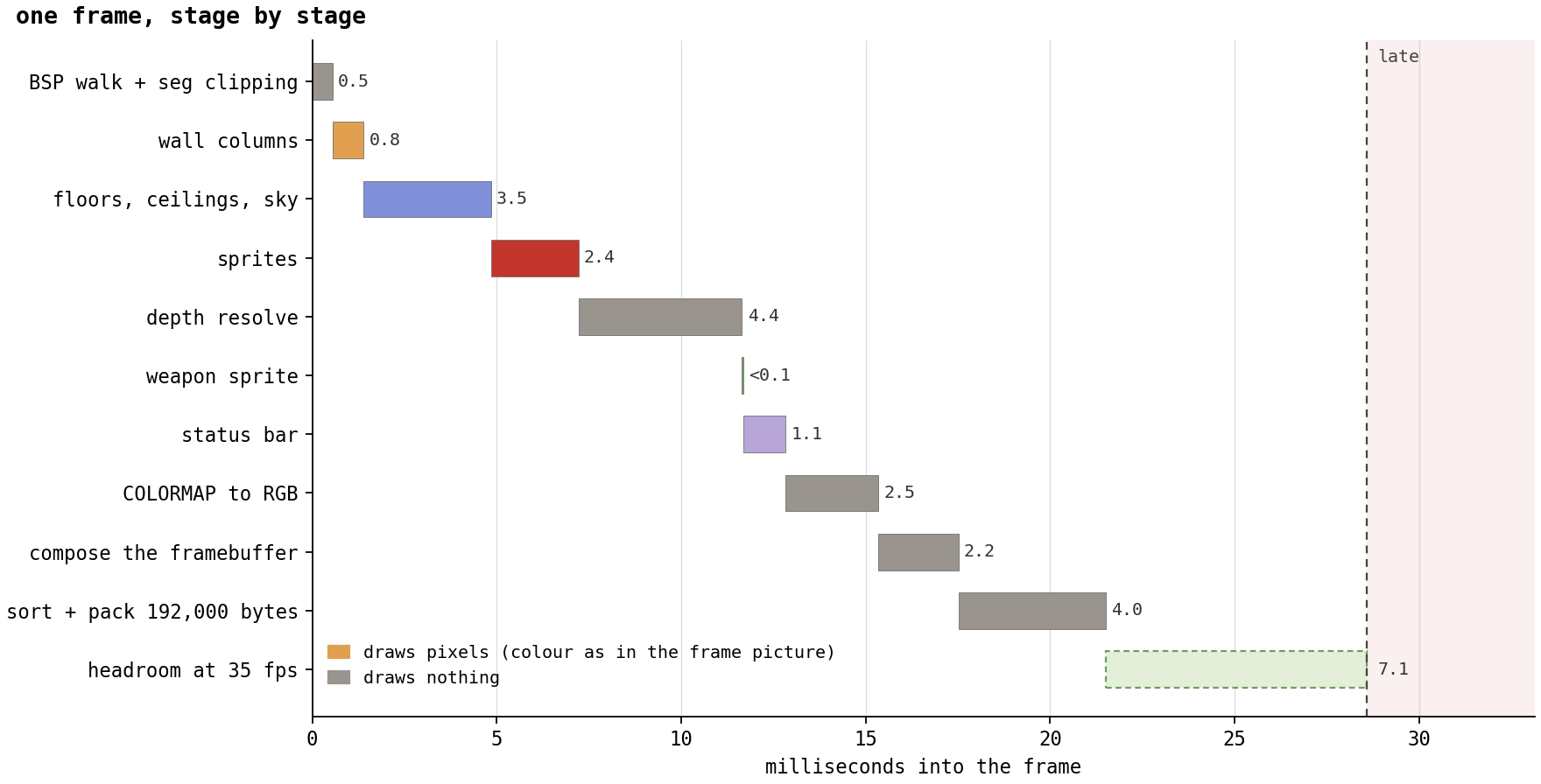
On my Laptop (Ryzen 7 PRO 7840U) I typically get about 60 FPS, but it drops down to 35 FPS on very busy scenes.

The most expensive parts of the pipeline are (unsurprisingly):

• rendering visplanes (where we have to emulate an iterative algorithm),
• depth resolve (which the original Doom successfully avoids in the first place),
• and everything that has to happen per pixel (e.g., colormap lookup, packing the framebuffer)

Where using a database is actually a good idea

Rendering Doom in a database is obviously a bad idea. But there are a few areas where it’s actually a good fit and I’m going to defend them to my death!

Everything is data

I previously didn’t expect how much I’d enjoy translating properties of items into a relational data set. For one, it makes it really easy to see what your game actually contains, but most importantly it’s also really easy to change.

The player’s shotgun is just a row:

doom=# SELECT name, ammo_type, ammo_per_shot, pellet_count,
doom-#        dmg_dice_count, dmg_dice_mult, max_range
doom-#   FROM weapon_defs WHERE name = 'shotgun';
  name   | ammo_type | ammo_per_shot | pellet_count | dmg_dice_count | dmg_dice_mult | max_range
---------+-----------+---------------+--------------+----------------+---------------+-----------
 shotgun | shells    |             1 |            7 |              3 |             5 |      2048
(1 row)

Seven pellets, each doing 3d5 damage.

Even the animation is data! Here’s the entire state machine of the shotgun:

doom=# SELECT state, seq_index AS seq, frame, tics,
doom-#        is_attack_frame AS shoots, refire_check AS refire
doom-#   FROM weapon_frames WHERE weapon_id = 3 ORDER BY state, seq_index;
 state | seq | frame | tics | shoots | refire
-------+-----+-------+------+--------+--------
 ready |   0 | A     |    1 | f      | f
 fire  |   0 | A     |    3 | f      | f
 fire  |   1 | A     |    7 | t      | f
 fire  |   2 | B     |    5 | f      | f
 fire  |   3 | C     |    5 | f      | f
 fire  |   4 | D     |    4 | f      | f
 fire  |   5 | C     |    5 | f      | f
 fire  |   6 | B     |    5 | f      | f
 fire  |   7 | A     |    3 | f      | t
 fire  |   8 | A     |    7 | f      | f
 flash |   0 | A     |    4 | f      | f
 flash |   1 | B     |    3 | f      | f
(12 rows)

Properties of things just being stored in a table also makes it really easy to mod everything. Take a look at the following clip where I’m frustrated I’m not doing enough damage, and just mod the shotgun to shoot 500 pellets at once at a higher spread!

Of course, we could have also just stored everything in files in e.g. JSON but that means

1. constraints aren’t verified at modification time and
2. We’d have to reload for changes to take effect.

Multiplayer almost comes for free

Well, now we went through all of this hassle to port over Doom to SQL and haven’t even taken advantage of the biggest strength of a database: You get a multiplayer server for free! Hear me out, we get a lot of stuff traditional game devs have to build themselves for free:

• Authentication
• Concurrency control
• Access control
• Consistent snapshots of the game state
• Binary wire protocol

A separate Python referee script drives the shared 35 Hz clock and rotates the map. The player’s clients online supply the input.

The part I like the most, though, is atomicity: Whenever we run a game tic, we can just say begin transaction, and commit in the end. Every player (Doom deathmatch supports up to 4) still gets a consistent view, either the way the world looked like before the tic transaction was started, or after it fully committed. No partially applied updates, physics bugs, or disagreements over whether the rocket actually hit.

The second part that was surprisingly elegant was access control. While sqldoom itself has about 110 tables and just over 100 functions, the four player roles are only allowed to interact with it through a few well-defined API functions. We just revoke access to everything else!

The input function that takes input from a player is a good example:

CREATE OR REPLACE FUNCTION api_input(
  p_fwd real, p_strafe real, p_run boolean, p_turn real,
  p_fire boolean, p_weapon integer, p_use boolean) RETURNS integer
LANGUAGE cedarscript SECURITY DEFINER AS $doom$
INSERT INTO mp_inputs
SELECT mp.map_id, mp.player_thing_id,
       LEAST(1.0, GREATEST(-1.0, COALESCE(p_fwd, 0)))::real,
       LEAST(1.0, GREATEST(-1.0, COALESCE(p_strafe, 0)))::real,
       [...]
FROM mp_players mp WHERE mp.role_name = session_user::text;
return 1;
$doom$;

While the function is allowed to make changes to tables (security definer), the player is only allowed to call the function. The only knobs they have is: Forward momentum (w/s pressed?), strafe (a/d pressed?), are they running?, turning via mouse?, is the fire button pressed?, which weapon is selected?, and do they try to press a button/open a door (spacebar)? We don’t even have to trust the player’s input values: The function is clamping the inputs to allowed values.

Multiplayer performance is also surprisingly good: 3 cores per client give stable 35 FPS, and the game tic still stays well below budget. Add an additional core for the tic driver and a 16 core machine is well equipped to run an original -altdeath doom deathmatch.

The public instance rotates through Episode 1 maps with a new map coming up every 10 minutes. If all four slots are occupied, you can still query the live match from the SQL console. Play, or query the live match →

Bonus: Compiling SQL

Surely a database written in C++ interpreting SQL is insanely inefficient and can’t come close to C? Probably not, but I wanted to evaluate how far off it really is.

CedarDB is a compiling database system: Every complex query is (through multiple steps) lowered to LLVM IR and then compiled to machine code. So I asked myself the question: How does that generated machine code differ from the original compiled linux_doom C code?

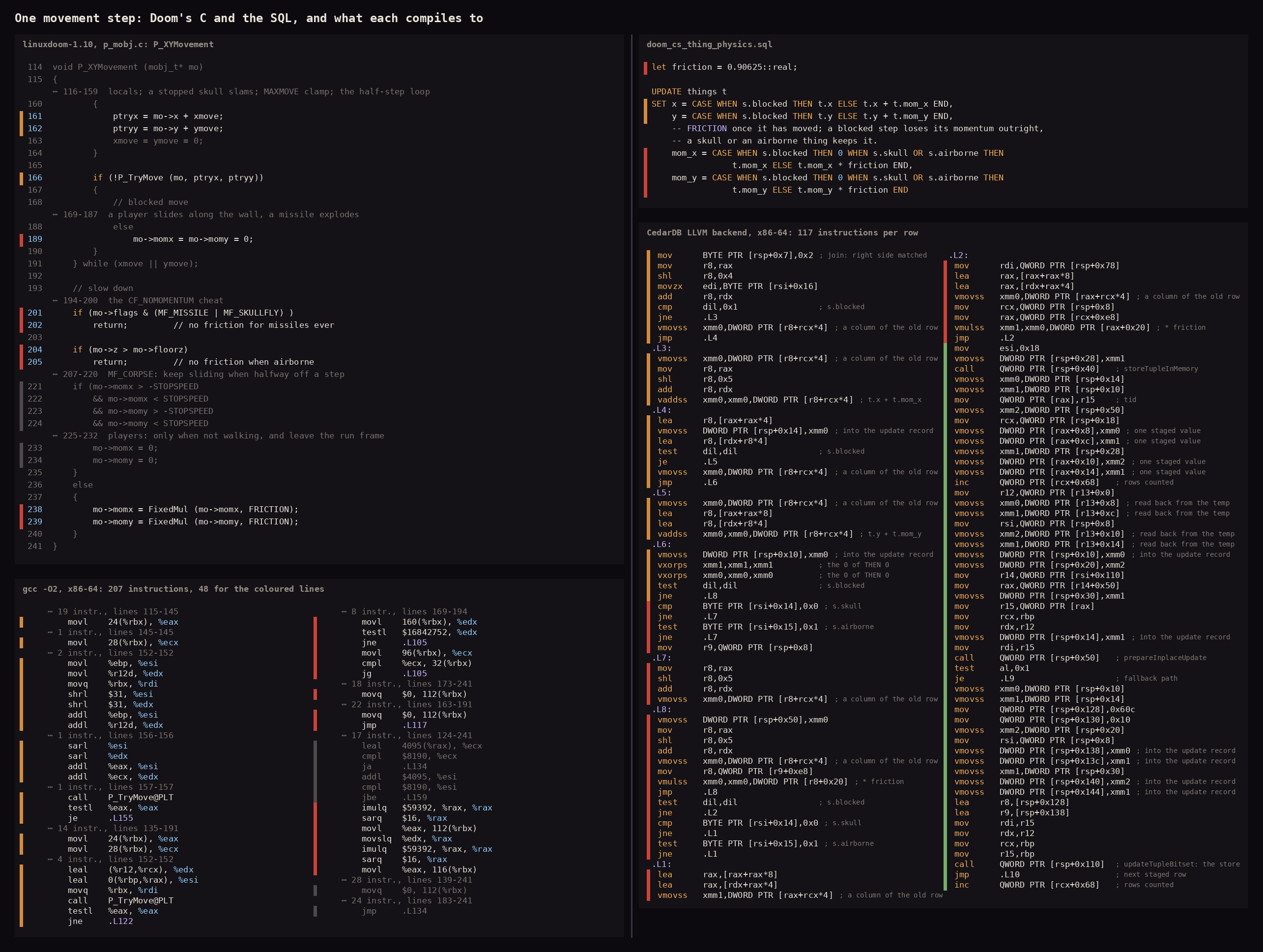
The upper half shows an object’s movement logic and how it’s influenced by momentum. The left side is the original doom source code, the right side shows the SQLDoom implementation. The comparison isn’t one-to-one since the logic is spread out a little bit differently, but the C code compiles to 48 instructions while SQLDoom takes 117 instructions. 42 of these additional instructions are actually storing the result in a table again (green lines), which C obviously doesn’t have to do. So it’s worse, don’t get me wrong, but it really isn’t that much worse for how many layers of abstraction are usually between SQL and your CPU. For something that started as SQL and passed through a query optimizer before reaching LLVM, I found the gap surprisingly small.

John Carmack was a genius.

I mean, compare SQLDoom against its Wolfenstein 3D-like predecessor DOOMQL

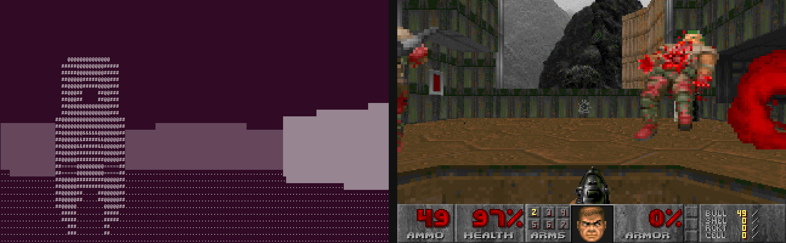
Both use the same engine, and same constraints: SQL in, bitmap out. And don’t get me wrong, DOOMQL’s primitive raycasting approach is awesome - much easier to formulate in SQL and not as many dependencies between steps - a much better fit for SQL’s set-based processing.

But it turns out that the “best fit” is not always the one with the best results. SQLDoom’s BSP-tree approach is much faster and its visual fidelity is a lot higher at the same time. All because John Carmack thought really hard about how much you can get out of your 486 with a little bit of smoke and mirrors.

And, to be honest, CedarDB also caught up. Back when I built DOOMQL, the engine was quite a bit slower and we didn’t have a role-based access system yet.

How to Run it Yourself

It’s on Github at github.com/cedardb/sqldoom.

You need three things:

1. CedarDB Community Edition,
2. Python with psycopg2 and pygame,
3. and a Doom IWAD which I can’t give you. The shareware doom1.wad is freely redistributable (apt install doom-wad-shareware) and is enough to play episode 1, and the retail WADs work if you own them.

From then on just follow the README and you should have your own SQLDoom running in no time!

Or, if that all sounds like too much work, just join a match on the public instance: